CCD Camera Gain Measurement

Tech Note: Pixel Response Effects on CCD Camera Gain Calibration

Author: Michael Newberry, Ph.D., Mirametrics, Inc.

August 1996

Overview

The gain of a CCD camera is the conversion between the number of electrons ("e-") recorded by the CCD and the number of digital units ("counts") contained in the CCD image. It is useful to know this conversion for evaluating the performance of the CCD camera. Since quantities in the CCD image can only be measured in units of counts, knowing the gain permits the calculation of quantities such as readout noise and full well capacity in the fundamental units of electrons. The gain value is required by some types of image deconvolution such as Maximum Entropy since, in order to correctly handle the statistical part of the calculation, the processing needs to convert the image into units of electrons. Calibrating the gain is also useful for detecting electronic problems in a CCD camera, including gain change at high or low signal level, and the existence of unexpected noise sources.

This White Paper develops the mathematical theory behind the gain calculation and shows how the mathematics suggests ways to measure the gain accurately. This note does not address the issues of basic image processing or CCD camera operation, and a basic understanding of CCD bias, dark and flat field correction is assumed.

CCD Camera Gain

The gain value is set by the electronics that read out the CCD chip. Gain is expressed in units of electrons per count. For example, a gain of 1.8 e-/count means that the camera produces 1 count for every 1.8 recorded electrons. Of course, we cannot split electrons into fractional parts, as in the case for a gain of 1.8 e-/count. What this number means is that 4/5 of the time 1 count is produced from 2 electrons, and 1/5 of the time 1 count is produced from 1 electron. This number is an average conversion ratio, based on changing large numbers of electrons into large numbers of counts. Note: This use of the term "gain" is in the opposite sense to the way a circuit designer would use the term since, in electronic design, gain is considered to be an increase in the number of output units compared with the number of input units.

It is important to note that every measurement you make in a CCD image uses units of counts. Since one camera may use a different gain than another camera, count units do not provide a straightforward comparison to be made. For example, suppose two cameras each record 24 electrons in a certain pixel. If the gain of the first camera is 2.0 and the gain of the second camera is 8.0, the same pixel would measure 12 counts in the image from the first camera and 3 counts in the image from the second camera. Without knowing the gain, comparing 12 counts against 3 counts is pretty meaningless.

Before a camera is assembled, the manufacturer can use the nominal tolerances of the electronic components to estimate the gain to within some level of uncertainty. This calculation is based on resistor values used in the gain stage of the CCD readout electronics. However, since the actual resistance is subject to component tolerances, the gain of the assembled camera may be quite different from this estimate. The actual gain can only be determined by actual performance in a gain calibration test. In addition, manufacturers sometimes do not perform an adequate gain measurement. Because of these issues, it is not unusual to find that the gain of a CCD camera differs substantially from the value quoted by the manufacturer.

Background

The signal recorded by a CCD and its conversion from units of electrons to counts can be mathematically described in a straightforward way. Understanding the mathematics validates the gain calculation technique described in the next section, and it shows why simpler techniques fail to give the correct answer.

This derivation uses the concepts of "signal" and "noise". CCD performance is usually described in terms of signal to noise ratio, or "S/N", but we shall deal with them separately here. The signal is defined as the quantity of information you measure in the image—in other words, the signal is the number of electrons recorded by the CCD or the number of counts present in the CCD image. The noise is the uncertainty in the signal. Since the photons recorded by the CCD arrive in random packets (courtesy of nature), observing the same source many times records a different number of electrons every time. This variation is a random error, or "noise" that is added to the true signal. You measure the gain of the CCD by comparing the signal level to the amount of variation in the signal. This works because the relationship between counts and electrons is different for the signal and the variance. There are two ways to make this measurement:

Measure the signal and variation within the same region of pixels at many intensity levels.
Measure the signal and variation in a single pixel at many intensity levels.

Both of these methods are detailed in section 6. They have the same mathematical foundation.

To derive the relationship between signal and variance in a CCD image, let us define the following quantities:

S_C	The signal measured in count units in the CCD image
S_E	The signal recorded in electron units by the CCD chip. This quantity is unknown.
N_C	The total noise measured in count units in the CCD image.
N_E	The total noise in terms of recorded electrons. This quantity is unknown.
g	The gain, in units of electrons per count. This will be calculated.
R_E	The readout noise of the CCD, in [electrons]. This quantity is unknown.
s _E	The photon noise in the signal N_E
s _o	An additional noise source in the image. This is described below.

We need an equation to relate the number of electrons, which is unknown, to quantities we measure in the CCD image in units of counts. The signals and noises are simply related through the gain factor as

and

These can be inverted to give

and

The noise is contributed by various sources. We consider these to be readout noise, R_E, photon noise attributable to the nature of light, , and some additional noise, , which will be shown to be important in in the following Section. Remembering that the different noise sources are independent of each other, they add in quadrature. This means that they add as the square their noise values. If we could measure the total noise in units of electrons, the various noise sources would combine in the following way:

The random arrival rate of photons controls the photon noise, _. Photon noise obeys the laws of Poissonian statistics, which makes the square of the noise equal to the signal, or . Therefore, we can make the following substitution:

Knowing how the gain relates units of electrons and counts, we can modify this equation to read as follows:

which then gives

We can rearrange this to get the final equation:

This is the equation of a line in which is the y axis, is the x axis, and the slope is 1/g. The extra terms are grouped together for the time being. Below, they will be separated, as the extra noise term has a profound effect on the method we use to measure gain. A better way to apply this equation is to plot our measurements with as the y axis and as the x axis, as this gives the gain directly as the slope. Theoretically, at least, one could also calculate the readout noise, , from the point where the line hits the y axis at = 0. Knowing the gain then allows this to be converted to a Readout Noise in the standard units of electrons. However, finding the intercept of the line is not a good method, because the readout noise is a relatively small quantity and the exact path where the line passes through the y axis is subject to much uncertainty.

With the mathematics in place, we are now ready to calculate the gain. So far, I have ignored the "extra noise term", . In the next 2 sections, I will describe the nature of the extra noise term and show how it affects the way we measure the gain of a CCD camera.

Crude Estimation of the Gain

Obtain images at different signal levels and subtract the bias from them. This is necessary because the bias level adds to the measured signal but does not contribute noise.
Measure the signal and noise in each image. The mean and standard deviation of a region of pixels give these quantities. Square the noise value to get a variance at each signal level.
For each image, plot Signal on the y axis against Variance on the x axis.
Find the slope of a line through the points. The gain equals the slope.

Is measuring the gain actually this simple? Well, yes and no. If we actually make the measurement over a substantial range of signal, the data points will follow a curve rather than a line. Using the present method we will always measure a slope that is too shallow, and with it we will always underestimate the gain. Using only low signal levels, this method can give a gain value that is at least "in the ballpark" of the true value. At low signal levels, the curvature is not apparent, though present. However, the data points have some amount of scatter themselves, and without a long baseline of signal, the slope might not be well determined. The curvature in the Signal - Variance plot is caused by the extra noise term which this simple method neglects.

The following factors affect the amount of curvature we obtain:

The color of the light source. Blue light is worse because CCD’s show the greatest surface irregularity at shorter wavelengths. These irregularities are described in Section 5.
The fabrication technology of the CCD chip. These issues determine the relative strength of the effects described in item 1.
The uniformity of illumination on the CCD chip.If the Illumination is not uniform, then the sloping count level inside the pixel region used to measure it inflates the measured standard deviation.

Fortunately, we can obtain the proper value by doing just a bit more work. We need to change the experiment in a way that makes the data plot as a straight line. We have to devise a way to account for the extra noise term, . If were a constant value we could combine it with the constant readout noise. We have not talked in detail about readout noise, but we have assumed that it merges together all constant noise sources that do not change with the signal level.

The Extra Noise Term in the Signal-Variance Relationship

The mysterious extra noise term, , is attributable to pixel-to-pixel variations in the sensitivity of the CCD, known as the flat field effect. The flat field effect produces a pattern of apparently "random" scatter in a CCD image. Even an exposure with infinite signal to noise ratio ("S/N") shows the flat field pattern. Despite its appearance, the pattern is not actually random because it repeats from one image to another. Changing the color of the light source changes the details of the pattern, but the pattern remains the same for all images exposed to light of the same spectral makeup. The importance of this effect is that, although the flat field variation is not a true noise, unless it is removed from the image it contributes to the noise you actually measure.

We need to characterize the noise contributed by the flat field pattern in order to determine its effect on the variance we measure in the image. This turns out to be quite simple: Since the flat field pattern is a fixed percentage of the signal, the standard deviation, or "noise" you measure from it is always proportional to the signal. For example, a pixel might be 1% less sensitive than its left neighbor, but 3% less sensitive than its right neighbor. Therefore, exposing this pixel at the 100 count level produces the following 3 signals: 101, 100, 103. However, exposing at the 10,000 count level gives these results: 10,100, 10,000, 10,300. The standard deviation for these 3 pixels is counts for the low signal case but is counts for the high signal case. Thus the standard deviation is 100 times larger when the signal is also 100 times larger. We can express this proportionality between the flat field "noise" and the signal level in a simple mathematical way: In the present example, we have k=0.02333. Substituting this expression for the flat field variation into our master equation, we get the following result:

With a simple rearrangement of the terms, this reveals a nice quadratic function of signal:

When plotted with the Signal on the x axis, this equation describes a parabola that opens upward. Since the Signal - Variance plot is actually plotted with Signal on the y axis, we need to invert this equation to solve for S_C:

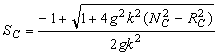
This final equation describes the classic Signal - Variance plot. In this form, the equation describes a family of horizontal parabolas that open toward the right. The strength of the flat field variation, k, determines the curvature. When k = 0, the curvature goes away and it gives the straight line relationship we desire. The curvature to the right of the line means that the stronger the flat field pattern, the more the variance is inflated at a given signal level. This result shows that it is impossible to accurately determine the gain from a Signal - Variance plot unless we know one of two things: Either 1) we know the value of k, or 2) we setup our measurements to avoid flat field effects. Option 2 is the correct strategy. Essentially, the weakness of the method described in Section 4 is that it assumes that a straight line relationship exists but ignores flat field effects.

To illustrate the effect of flat field variations, mathematical models were constructed using the equation above with parameters typical of commonly available CCD cameras. These include readout noise R_E = 15e- and gain g = 2.0 e- / Count. Three models were constructed with flat field parameters k = 0, k = 0.005, and k = 0.01. Flat field variations of this order are not uncommon. These models are shown in the figure below.

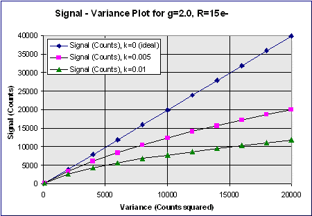
Increasing values of k correspond to progressively larger flat field irregularities in the CCD chip. The amplitude of flat field effects, k, tends to increase with shorter wavelength, particularly with thinned CCD's (this is why Section 4 recommends using a redder light source to illuminate the CCD). The flat field pattern is present in every image exposed to light. Clearly, it can be seen from the models that if one simply obtains images at different signal levels and measures the variance in them, then fitting a line through any part of the curve yields a slope lower than its true value. Thus the simple method of section 4 always underestimates the gain.

The best strategy for doing the Signal - Variance method is to find a way to produce a straight line by properly compensating for flat field effects. This is important by the "virtue of straightness": Deviation from a straight line is completely unambiguous and easy to detect. It avoids the issue of how much curvature is attributable to what cause. The electronic design of a CCD camera is quite complex, and problems can occur, such as gain change at different signal levels or unexplained extra noise at high or low signal levels. Using a "robust" method for calculating gain, any significant deviation from a line is a diagnostic of possible problems in the camera electronics. Two such methods are described in the following section.

In previous sections, the so-called simple method of estimating the gain was shown to be an oversimplification. Specifically, it produces a Signal - Variance plot with a curved relationship resulting from flat field effects. This section presents two robust methods that correct the flat field effects in the Signal - Variance relationship to yield the desired straight-line relationship. This permits an accurate gain value to be calculated. Adjusting the method to remove flat field effects is a better strategy than either to attempt to use a low signal level where flat field effects are believed not to be important or to attempt to measure and compensate for the flat field parameter k.

When applying the robust methods described below, one must consider some procedural issues that apply to both:

Both methods measure sets of 2 or more images at each signal level. An image set is defined as 2 or more successive images taken under the same illumination conditions. To obtain various signal levels, it is better to change the intensity received by the CCD than to change the exposure time. This may be achieved either by varying the light source intensity or by altering the amount of light passing into the camera. The illumination received by the CCD should not vary too much within a set of images, but it does not have to be truly constant.

Cool the CCD camera to reduce the dark current to as low as possible. This prevents you from having to subtract dark frames from the images (doing so adds noise, which adversely affects the noise measurements at low signal level). In addition, if the bias varies from one frame to another, be sure to subtract a bias value from every image.
The CCD should be illuminated the same way for all images within a set. Irregularities in illumination within a set are automatically removed by the image processing methods used in the calibration. It does not matter if the illumination pattern changes when you change the intensity level for a different image set.
Within an image set, variation in the light intensity is corrected by normalizing the images so that they have the same average signal within the same pixel region. The process of normalizing multiplies the image by an appropriate constant value so that its mean value within the pixel region matches that of other images in the same set. Multiplying by a constant value does not affect the signal to noise ratio or the flat field structure of the image.
Do not estimate the CCD camera's readout noise by calculating the noise value at zero signal. This is the square root of the variance where the gain line intercepts the y axis. Especially do not use this value if bias is not subtracted from every frame. To calculate the readout noise, use the "Two Bias" method and apply the gain value determined from this test. In the Two Bias Method, 2 bias frames are taken in succession and then subtracted from each other. Measure the standard deviation inside a region of, say 100x100 pixels and divide by 1.4142. This gives the readout noise in units of counts. Multiply this by the gain factor to get the Readout Noise in units of electrons. If bias frames are not available, cool the camera and obtain two dark frames of minimum exposure, then apply the Two Bias Method to them.

Method 1: Correct the flat field effects at each signal level

In this strategy, the flat field effects are removed by subtracting one image from another at each signal level. Here is the recipe:

For each intensity level, do the following:

Obtain 2 images in succession at the same light level. Call these images A and B.
Subtract the bias level from both images. Keep the exposure short so that the dark current is negligibly small. If the dark current is large, you should also remove it from both frames.
Measure the mean signal level S in a region of pixels on images A and B. Call these mean signals S_A and S_B. It is best if the bounds of the region change as little as possible from one image to the next. The region might be as small as 50x50 to 100x100 pixels but should not contain obvious defects such as cosmic ray hits, dead pixels, etc.
Calculate the ratio of the mean signal levels as r = S_A / S_B.
Multiply image B by the number r. This corrects image B to the same signal level as image A without affecting its noise structure or flat field variation.
Subtract image B from image A. The flat field effects present in both images should be cancelled to within the random errors.
Measure the standard deviation over the same pixel region you used in step 3. Square this number to get the Variance. In addition, divide the resulting variance by 2.0 to correct for the fact that the variance is doubled when you subtract one similar image from another.
Use the Signal from step 3 and the Variance from step 7 to add a data point to your Signal - Variance plot.
Change the light intensity and repeat steps 1 through 8.

Method 2: Avoid flat field effects using one pixel in many images.

This strategy avoids the flat field variation by considering how a single pixel varies among many images. Since the variance is calculated from a single pixel many times, rather than from a collection of different pixels, there is no flat field variation.

To calculate the variance at a given signal level, you obtain many frames, measure the same pixel in each frame, and calculate the variance among this set of values. One problem with this method is that the variance itself is subject to random errors and is only an estimate of the true value. To obtain a reliable variance, you must use 100’s of images at each intensity level. This is completely analogous to measuring the variance over a moderate sized pixel region in Method A; in both methods, using many pixels to compute the variance gives a more statistically sound value. Another limitation of this method is that it either requires a perfectly stable light source or you have to compensate for light source variation by adjusting each image to the same average signal level before measuring its pixel. Altogether, the method requires a large number of images and a lot of processing. For this reason, Method A is preferred. In any case, here is the recipe:

Select a pixel to measure at the same location in every image. Always measure the same pixel in every image at every signal level.

For each intensity level, do the following:

Obtain at least 100 images in succession at the same light level. Call the first image A and the remaining images i. Since you are interested in a single pixel, the images may be small, of order 100x100 pixels.
Subtract the bias level from each image. Keep the exposure short so that the dark is negligibly small. If the dark current is large, you should also remove it from every frame.
Measure the mean signal level S in a rectangular region of pixels on image A. Measure the same quantity in each of the remaining images. The measuring region might be as small as 50x50 to 100x100 pixels and should be centered on the brightest part of the image.
For each image S_i other than the first, calculate the ratio of its mean signal level to that of image A. This gives a number for each image, r_i = S_A / S_i.
Multiply each image i by the number r_i. This corrects each image to the same average intensity as image A.
Measure the number of counts in the selected pixel in every one of the images. From these numbers, compute a mean count and standard deviation. Square the standard deviation to get the variance.
Use the Signal and Variance from step 6 to add a data point to your Signal - Variance plot.
Change the light intensity and repeat steps 1 through 7.

Summary

We have derived the mathematical relationship between Signal and Variance in a CCD image which includes the pixel-to-pixel response variations among the image pixels. This "flat field" effect must be compensated or the calculated value of the camera gain will be incorrect. We have shown how the traditional "simple" method used for gain calculation leads to an erroneous gain value unless flat field effects are not considered. We have suggested 2 methods that correctly account for the flat field effect, and these should be implemented in camera testing procedures.