CPlotView:Plotting a Least Squares Fit
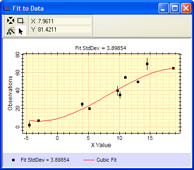
The following plot shows the result of a least squares fit to 10 points. Each point is the local group average of several points and the standard deviation among the points is shown as its error bar. The least square fit used optimal weighting in which the weight of each point is equal to the inverse of its variance. This plot shows 2 series in Overplot mode: Series 1 plots the square markers with error bars. Series 2 plots the polynomial fit evaluated at 100 points over the x range of the data. The script that produced this plot is listed below.
The script first enters the data to be plotted. In this case, the values were typed-in, but the data might also have been loaded form a text file or from a Mira table. Each of the 10 entries represents the group average and standard deviation of the grouped data. Three entries are given for x, y, and s. The value of s is the y direction standard deviation for the group of points at average coordinates x, y. The script defines a simple helper function to convert the standard deviation s into a weight using the inverse variance method and then uses it to compute the cubic polynomial fit. The data are then plotted in Series 1 and and the fit is evaluated at 100 points over the data range to create Series 2.
|
|
-- create the least squares fitting object |
|
|
-- fit a 4 term (cubic) polynomial |
|
|
-- add 10 data (x,y) points with y weights |
|
|
|
|
|
|
|
|
|
|
|
|
|
|
|
|
|
|
|
|
|
|
|
|
|
|
|
|
|
-- compute the least squares fit |
|
-- now plot the data points and their fit |
|
|
|
-- create a new CPlotView instance |
|
-- Plot the data points as markers |
|
|
|
-- add each point as a marker |
|
|
|
|
|
|
|
-- make a caption from the fit sigma and create the plot of data points: |
|
|
|
|
|
|
|
|
|
-- clear out existing plot points |
|
-- Plot the fit using 100 line segments over the range of data: |
|
|
|
|
|
|
|
|
|
-- run through the x range in 100 steps |
|
|
-- plot a line between points |
|
|
|
|
|
-- add evaluation points as a new series |
|
|
-- show both series using overplot mode |
CPlotView class, Add , CLsqFit class
Mira Pro x64 Script User's Guide, Copyright Ⓒ 2023 Mirametrics,
Inc. All Rights Reserved.