
 This
overview describes
some of the interactive visualization and measurement tools in Mira Pro and
Mira Pro x64. This
presentation is derived from topics in the Mira
User's Guide document. Additional tutorials are provided in the
program help and the Mira
User's Guide.
This
overview describes
some of the interactive visualization and measurement tools in Mira Pro and
Mira Pro x64. This
presentation is derived from topics in the Mira
User's Guide document. Additional tutorials are provided in the
program help and the Mira
User's Guide.
NOTE: All features described here are included in Mira Pro x64. Some features are not available for regular Mira Pro. See the Product Comparison matrix for details.
NOTE: Some features described here are available in Mira Pro Ultimate Edition, but not in Mira Pro. See the Product Comparison matrix for details.
Contents
| Tutorial | |
| Glossary of Terms | |
| Other Information |
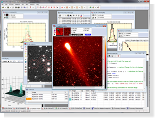
Tutorial
This tutorial describes how to display an image or image set and make some interactive adjustments, plots, and measurements. This tutorial does not discuss the rich collection of powerful processing tools provided by Mira Pro.
Note: The screen pictures shown below are "thumbnails". To see an image full size, click on the image. After that, click the browser's "Back" button to return to this tutorial.
Opening an Image
 Start Mira in the usual way.
Click File on the main
menu bar, then Open... in the File menu (we will refer
to this and other menu commands like File
> Open). This command displays an Open dialog similar to the
one shown at right (Remember, click on the image to view it full size, then
use the "Back" button to return to this tutorial).
Start Mira in the usual way.
Click File on the main
menu bar, then Open... in the File menu (we will refer
to this and other menu commands like File
> Open). This command displays an Open dialog similar to the
one shown at right (Remember, click on the image to view it full size, then
use the "Back" button to return to this tutorial).
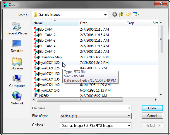
Navigate to the Sample Images folder. If using Mira version 8, this is inside your "documents" folder which usually is named "My Documents" . For generality, here we will call your documents area <Documents>, whatever its name. If you are running Mira Pro x64 or Mira Pro, this location will be one of the following:
<Documents>\Mira Pro x64\Sample Data
<Documents>\Mira Pro\Sample Data
If using Mira version 7, the images folder is located in your "My Pictures" folder, depending on whether you are running Mira Pro x64 or Mira Pro:
My Pictures\Mirametrics\Mira Pro 7 UE\Sample Images
My Pictures\Mirametrics\Mira Pro 7\Sample Images
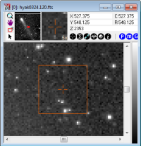
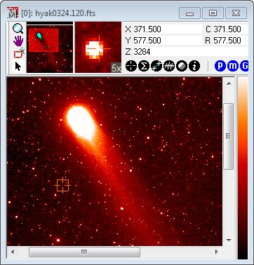
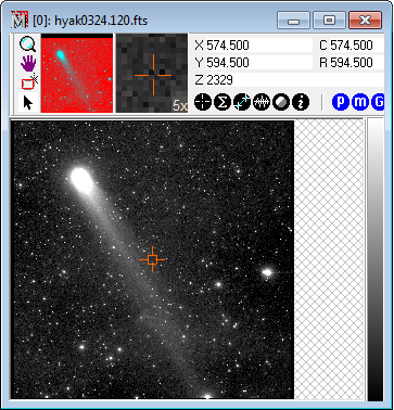 In the File Open
dialog, click on hyak0324.120.fts
to select it, then click [Open]. The image is
opened into an Image Window like the one shown at right. Note that the
image appears small because it was automatically scaled to fit the screen. Image scaling is set in the Preferences > Image dialog (Ctrl+R);
this example uses "Display Entire Image". Displaying the entire
image may shrink it to the point where some buttons on the Image Toolbar may
not be shown, but you can re-size the window if needed. [The Image Toolbar can be disabled; see the Mira User's Guide.]
The image Toolbar also displays world coordinates if the image is
so-calibrated.
In the File Open
dialog, click on hyak0324.120.fts
to select it, then click [Open]. The image is
opened into an Image Window like the one shown at right. Note that the
image appears small because it was automatically scaled to fit the screen. Image scaling is set in the Preferences > Image dialog (Ctrl+R);
this example uses "Display Entire Image". Displaying the entire
image may shrink it to the point where some buttons on the Image Toolbar may
not be shown, but you can re-size the window if needed. [The Image Toolbar can be disabled; see the Mira User's Guide.]
The image Toolbar also displays world coordinates if the image is
so-calibrated.
|
Note |
If a FITS format image opens upside down, open the File Open dialog and check the Flip FITS Images option, then re-open the image. This option can also be set on the Other Preferences page. |
Adjusting the Image
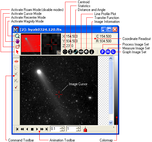 Along the top of the Image Window is an
image command center called
the Image Toolbar. The toolbar and other window components are
defined in the picture at right (click to enlarge). The dynamic (changing) parts
of the Image Toolbar are the two Auxiliary Image Views and the Image Coordinate
Display panels. The auxiliary views show a thumbnail that indicates the
currently visible region and a magnified view that tracks the mouse pointer.
The Coordinate Display section also tracks the mouse pointer, displaying both
column and row position in the image (C and R) as well as the
pixel value Z, and the World Coordinates X, and Y. World
Coordinates refers to Right Ascension and Declination. This image has no World
Coordinate System (WCS) calibration so (X,Y) equals (C,R).
Along the top of the Image Window is an
image command center called
the Image Toolbar. The toolbar and other window components are
defined in the picture at right (click to enlarge). The dynamic (changing) parts
of the Image Toolbar are the two Auxiliary Image Views and the Image Coordinate
Display panels. The auxiliary views show a thumbnail that indicates the
currently visible region and a magnified view that tracks the mouse pointer.
The Coordinate Display section also tracks the mouse pointer, displaying both
column and row position in the image (C and R) as well as the
pixel value Z, and the World Coordinates X, and Y. World
Coordinates refers to Right Ascension and Declination. This image has no World
Coordinate System (WCS) calibration so (X,Y) equals (C,R).
We now want to magnify the image. If the mouse has a
thumbwheel, and the image window is active (on top; has focus), we can rotate
the wheel to magnify the image. Otherwise, the quickest way is to use Magnify
Mode. Move the mouse onto
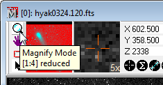 the button at the extreme top left corner of the
window and let the mouse hover over the button. This is the Magnify Mode
button. If you click it, Mira changes into Magnify Mode in which left mouse
clicks on the image magnify it at that point. If you let the mouse hover over
the button, a Tooltip pops up as shown at far left.
the button at the extreme top left corner of the
window and let the mouse hover over the button. This is the Magnify Mode
button. If you click it, Mira changes into Magnify Mode in which left mouse
clicks on the image magnify it at that point. If you let the mouse hover over
the button, a Tooltip pops up as shown at far left.
This is a special kind of Tooltip that shows a triangle on the right side. This is an Expanding Tooltip, which can display additional text. To see more text, click on the triangle at the right end of the tip. The Magnify Tooltip tells you not only what the Magnify button does, but also that the image is reduced by 4 times. If you click on this Tooltip you will see expanded information that tell you how to use magnify mode. Many Mira controls have Expanding Tooltips. As with the Magnify button, many of the other buttons on the Image Toolbar have Tooltips that tell you about the current state of the command.
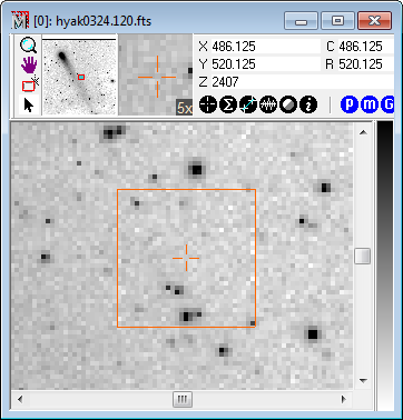
Next we will zoom the image from 1:4 up to 4:1 (this changes the magnification by these 4 steps: 1:2, 1:1, 2:1, and 4:1. You can zoom the image using either of the following methods:
-
 Click on the magnifying class on the Image Toolbar, then
point the crosshair pointer at the middle if the image cursor and click 4
times. [To de-zoom, press [Shift] and click 4 times.]
Click on the magnifying class on the Image Toolbar, then
point the crosshair pointer at the middle if the image cursor and click 4
times. [To de-zoom, press [Shift] and click 4 times.]
- Without clicking on the magnifying glass, roll the mouse thumbwheel forward 4 steps. [To de-zoom, roll the thumbwheel backward 4 steps.]

The result of magnifying the image is shown at right.
Note that the magnification done by clicking on the image always occurs centered at the location of the crosshair on the image. You also can magnify the image using commands in the right-click context menu of the image, or using commands in the View menu; these commands always magnify the image about the center of the image.
Using the Image Cursor
In the previous figure, the image shows a large red square
with a small central crosshair. This rectangle is the Image Cursor, a
resizable tracking cursor used for defining positions and rectangular regions
on the image. The Image Cursor is used by a number of Mira commands and
interactive tools. The image cursor is connected to the image's pixel
coordinate system rather than the computer screen. The edges and center are
always reported to Mira internally as actual (fractional) pixel coordinates.
Now, we will change to Cursor mode to be able to adjust the Image Cursor. Click
![]() to switch to Cursor Mode. (As usual with
cursor command modes, you switch out by clicking
to switch to Cursor Mode. (As usual with
cursor command modes, you switch out by clicking
![]() to return to Roam Mode.) You can also
change modes by right clicking on the image to open the Image Context Menu
instead of the button commands.
to return to Roam Mode.) You can also
change modes by right clicking on the image to open the Image Context Menu
instead of the button commands.
There are two other ways to adjust the image cursor:
- In any mode, hold down Shift and click the mouse on a target position to move the cursor. This does not enable Cursor mode.
- Use Ctrl+D to switch in and out of Cursor Mode.
To move the Image Cursor while Cursor Mode is enabled, simply click on the image. The Image Cursor responds to "[left] mouse button down" by locking onto the mouse pointer, wherever it may be. Thus you can position or drag the Image Cursor by having the mouse button down. To resize the Image Cursor, move the mouse pointer over an edge or corner to see the pointer icon change to a double arrow. Then mouse down on that point and stretch the Image Cursor as desired. These moving and stretching operations work only while in Cursor Mode. You should use these actions to position the Image Cursor on a place of interest in the image. If the Image Cursor is lost somewhere outside the visible portion of the image, say when it is highly magnified, just enter Cursor Mode and mouse down somewhere on the image. That will relocate it to the point where you clicked. You can also position the Image Cursor at an exact coordinate (pixel or world) using the Go To Coordinate command in the View > Coordinates menu or the Image Context Menu. The Go To Coordinate window stays open so you can dock it near the edge of the screen to use as needed.
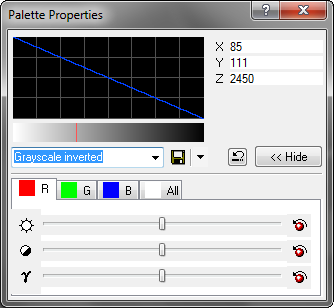
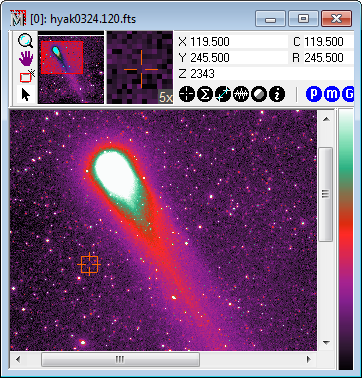
Adjusting the Image Palette
Let's play with the Image Palette. The right border of the Image Window shows the relationship between image "luminance" (intensity, pixel value, count, ADU, etc.) and the color assigned to it by the Image Palette. This region, which looks like a grayscale ramp in this example, is called the Image Colormap. The Colormap shows the current palette. To change the palette, move the mouse pointer onto the Colormap "hot zone" so that the pointer changes to a red/blue yin-yang icon; this indicates that palette commands are available by clicking the mouse in this "hot zone" if the colormap (Note: another type of display adjustment is made using commands in the View > Transfer Function menu).
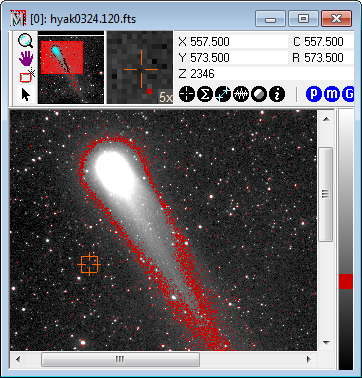
To change the image to that seen at left, below, the palette was inverted by switching the palette to "Grayscale Inverted" in the Palette Manager (at right, below). The various ways to change the palette are described in the table below the pictures.
Palette Adjustment Commands:
- To stretch any palette's contrast and brightness, "mouse down" on the Colormap, and move the pointer around the screen while keeping the mouse button down.
- To adjust the palette gamma and brightness, instead of contrast and brightness, press the [Shift] key, then "mouse down" on the Colormap and drag the pointer around the screen while keeping the mouse button down.
- To invert any palette in effect, use the View > Palette > Invert command in the main menu.
- To view palette details or switch palettes, double click on the Colormap to open the Palette Properties dialog.
- To reset the palette to its default settings, right double click on the Colormap.
A transfer function is a prescription that describes how to "slice" the luminance range of an image into some number of levels for display. To each level is applied a color (or gray shade) entry from a palette. The transfer function is applied to luminance (i.e., non-color) images. A palette is applied to both luminance and color images. By changing either the transfer function or the palette assignments, you can change the way an image is displayed. Neither the transfer function nor palette affects the actual pixel values; they are both just display enhancements. You can prove this to yourself by adjusting the palette and noting the pixel values as you roam the mouse pointer around the image — there is no change in values despite the change in appearance. All measurements, processing, and plotting are also independent of transfer function and palette settings. For more information, see Image Palettes in the Mira User's Guide.
Double click on the Colormap to open the Palette Properties dialog. Underneath the palette graph is a drop box containing the names of different palettes. This drop box and its buttons to the right are called a Profile Control. The grayscale palette is the default when an image is opened, and it performs a direct mapping of gray shade or color assignments to the image values. You can also apply false colors to the transfer function levels using a "pseudocolor" type palette. Pseudocolor allows certain image features to be enhanced at the expense of others and represents a powerful say of visualizing images. In the drop list, select a different palette name and notice how the image window having focus changes to apply it immediately. After loading a palette, you can stretch its contrast and brightness and watch the palette change. The views below were made using 3 of the 27 standard palettes: From the left, these are "Pseudocolor 3", "Flame", and "Level Slice" (the palette was stretched to highlight a narrow range of brightness).
Making Plots
Mira Pro allows you to quickly and easily make several types of plots of your image data. Depending on the type of plot, the pixels to be plotted are taken wither from the position and size of the image cursor or from drawing on the image. If you do not move the Image Cursor between plots, this software design means that you can get easily column, row, and radial brightness plots all at exactly the same coordinate. Plots can use either "Pixel" coordinates or, if the image has a World Coordinate System calibration then the plot also can use World Coordinates. When a world calibration involves right ascension and declination, a world coordinate mode plot uses distance in arc seconds. In addition to the plots discussed here, Mira Pro provides light curve plots as part of the Photometry package.
To illustrate plotting, we will open a different image and create some plots from it. Using the File > Open dialog, open the image named BL-CAM.fts.
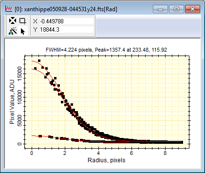
Radial Profile and FWHM Measurement
The first plot we make will show the radial brightness profile and
provide a measurement the Full Width at Half Maximum ("FWHM") of a point source.
This command works with the Image Cursor (see above). Zoom-in on the star near coordinate (764,608), as shown at left, below.
You do not have to move exactly onto the object because Mira will
automatically center on the star while creating the plot. To quickly move
the image cursor to a point, use the Shift+Click strategy:
Hold down the Shift
key and click the mouse pointer where you want to move it — the Shift+Click method allows you to move the cursor
to a point, regardless of the current cursor mode, without having to switch
to Cursor Mode. Now
create the plot by clicking the
![]() button
in Mira Pro or the
button
in Mira Pro or the
![]() button in Mira Pro x64. This plot is shown below.
button in Mira Pro x64. This plot is shown below.


In Mira Pro x64, radial profile
preferences can be set from the drop menu using the down arrow on the right
side of the
![]() button.
button.
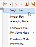
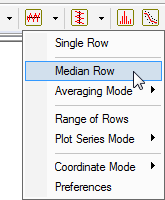
Row Profile Plots
This type of plot, and the related Column Profile Plot, also use the Image Cursor and are called "cursor plots". Row and Column plots come in different flavors (see the drop-menu below, left), including a single row (or column), an average over a range of rows (or columns), or all of the individual rows (or columns) inside the image cursor. You select the rows or columns to plot by positioning and resizing the Image Cursor. The general strategy for making cursor plots is first to position and resize the Image Cursor to mark the target pixels, then click the command to make the plot.
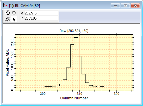
First, we will plot a Single Row through
the center of the image cursor. Click the
![]() button to
create the plot (or open a menu and click "Single Row"). This creates the
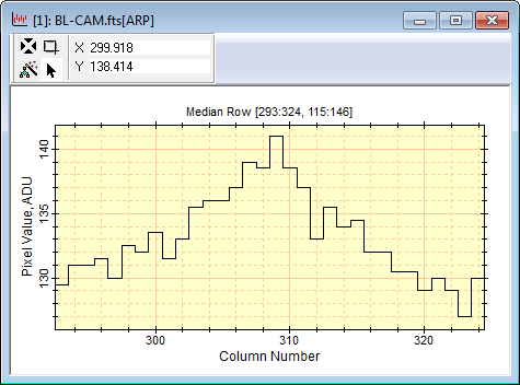
plot shown next to the drop-menu. Now, let's make a single row plot that
shows the median brightness inside the Image Cursor. To do this, select
"Median Row" from the drop-down menu or after right-clicking on the image.
If the menu does not show "Median Row", select it from the "Averaging Mode"
option, then re-open the menu and use the Median Row
command. These results are shown at right, below.
button to
create the plot (or open a menu and click "Single Row"). This creates the
plot shown next to the drop-menu. Now, let's make a single row plot that
shows the median brightness inside the Image Cursor. To do this, select
"Median Row" from the drop-down menu or after right-clicking on the image.
If the menu does not show "Median Row", select it from the "Averaging Mode"
option, then re-open the menu and use the Median Row
command. These results are shown at right, below.
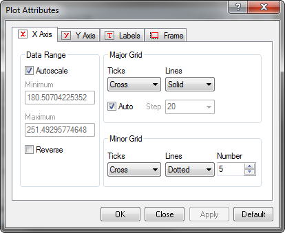 All of the plot attributes: scale, ticks, fonts, colors,
line color and thickness, etc., can be changed. To do this, right click on the plot to open the pop-up
menu and select "Plot Attributes..." to open the dialog shown
at right.
Change some of the settings, then click "Apply". To make the settings
permanent, for all future Plot windows, click "Default".
All of the plot attributes: scale, ticks, fonts, colors,
line color and thickness, etc., can be changed. To do this, right click on the plot to open the pop-up
menu and select "Plot Attributes..." to open the dialog shown
at right.
Change some of the settings, then click "Apply". To make the settings
permanent, for all future Plot windows, click "Default".
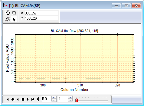
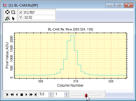
Next,
we will create a plot showing all rows inside the Image Cursor. To do this,
you may wish to first switch to adjust the Image Cursor (switch to Cursor
Mode using the
![]() on the
Image Window, adjust the cursor then click
on the
Image Window, adjust the cursor then click
![]() to change
to the default "Roam" mode). To make the plot, select "Range of Rows" as
shown at left, below. The range of rows plots all rows inside the image
cursor in a single plot window. Two Plot Modes are
available for displaying all rows: You can use Animate mode
in which you can scroll through the individual row plots, or
Overplot mode which displays all rows on the same set of axes. The
left and middle pictures below show Animate Mode with different rows
selected using the red thumb at bottom of the window. The colors of the
various plot series can be set before all future plots are created using the
Plot Preferences dialog (Ctrl+R, then select the "Plot"
tab, followed by "Default").
to change
to the default "Roam" mode). To make the plot, select "Range of Rows" as
shown at left, below. The range of rows plots all rows inside the image
cursor in a single plot window. Two Plot Modes are
available for displaying all rows: You can use Animate mode
in which you can scroll through the individual row plots, or
Overplot mode which displays all rows on the same set of axes. The
left and middle pictures below show Animate Mode with different rows
selected using the red thumb at bottom of the window. The colors of the
various plot series can be set before all future plots are created using the
Plot Preferences dialog (Ctrl+R, then select the "Plot"
tab, followed by "Default").
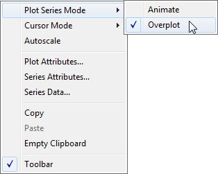
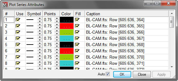
Next we will switch to Overplot mode. To do this, right-click on the plot and select "Plot Series Mode > Overplot" from the pop-up menu. This menu and the resulting plot are shown below.
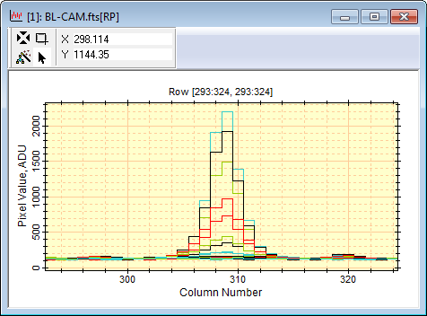
The Plot Mode can be selected globally, to control the way the plot window opens, by selecting Animate or Overplot mode from one of the plot button drop menus. To change the properties of the individual plot series, open the Plot Context Menu shown above and click the "Series Attributes" command. The Plot Series Attributes dialog shown below can be opened from any Plot window. Use this to change the attributes of one or any number of plot series drawn in the current Plot window. To change more than one series, see instructions in the Mira User's Guide.
Histogram Plot
Histogram plots show the frequency of pixel values that
occur inside the Image Cursor. The histogram can be
created using the
![]() button on the main toolbar or by using the View > Plot > Histogram
command from the main menu (or right-click on the image to open an alternative Plot menu). In
the BL-CAM.fts image, move the Image Cursor off the
star and into a blank area of sky background above the star. Then click
button on the main toolbar or by using the View > Plot > Histogram
command from the main menu (or right-click on the image to open an alternative Plot menu). In
the BL-CAM.fts image, move the Image Cursor off the
star and into a blank area of sky background above the star. Then click
![]() to
create the plot shown at left, below.
to
create the plot shown at left, below.

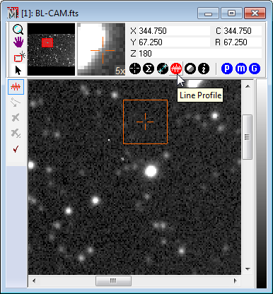
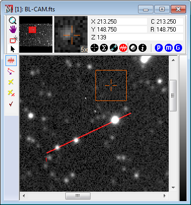
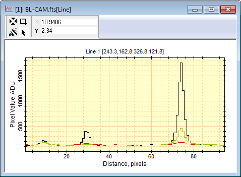
Line Profile Plot
This type of plot shows the brightness profile along a
line drawn on the image. Unlike the Row and Column plots, which get the
pixel sample from the
Image Cursor, this plot command operates from a toolbar and is
created by manually drawing a line on the image. The BL-CAM.fts image below shows the
Mira Image Window after clicking the
![]() button on the
Image
Toolbar (red-highlighted). Notice that the Line Profile toolbar has opened along the left
margin of the Image Window. This, and other such toolbars, automatically
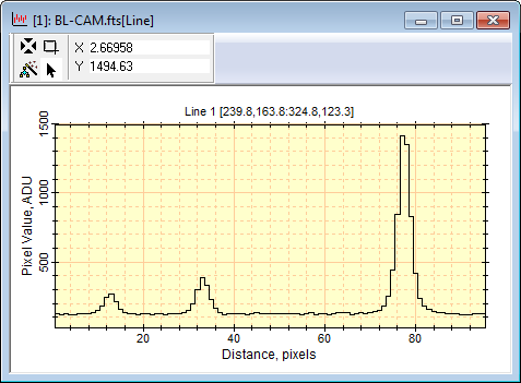
open in marking mode. To create the plot, mouse down at the starting point
(lower left, here), drag to the ending point (upper right), and release the
mouse there. The plot is shown at right, below.
button on the
Image
Toolbar (red-highlighted). Notice that the Line Profile toolbar has opened along the left
margin of the Image Window. This, and other such toolbars, automatically
open in marking mode. To create the plot, mouse down at the starting point
(lower left, here), drag to the ending point (upper right), and release the
mouse there. The plot is shown at right, below.
Similar to the "Range of Rows" command described above, the Line
Profile tool allows multiple plots to be drawn on the
 same
set of axes. To do this, click
same
set of axes. To do this, click
![]() to switch to Move Mode. Then
mouse-down on the line you have drawn and drag it to
a
new coordinate. When you release the mouse button, the new brightness
profile is added to the plot window you created. As described above for the
"Range of Rows" plot, you can select Animate or
Overplot mode to control
which lines are displayed. A plot sequence number is
shown at the starting point. The plot window at right shows the result of
moving the line vector 2 times in Move Mode.
to switch to Move Mode. Then
mouse-down on the line you have drawn and drag it to
a
new coordinate. When you release the mouse button, the new brightness
profile is added to the plot window you created. As described above for the
"Range of Rows" plot, you can select Animate or
Overplot mode to control
which lines are displayed. A plot sequence number is
shown at the starting point. The plot window at right shows the result of
moving the line vector 2 times in Move Mode.
The caption inside the Plot window shows the image coordinates at the line endpoints as [col1:col2, row1:row2]. If your image had a world coordinate calibration. all plots could be created using world coordinates. If you have plotted multiple line profiles then, in Animate mode, each plot caption lists the unique coordinates of its endpoints.
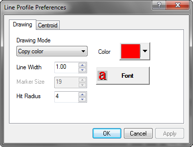 The properties of the line profile drawing can be set by
opening the Line Profile Preferences dialog as shown at
right. Do this by clicking the
The properties of the line profile drawing can be set by
opening the Line Profile Preferences dialog as shown at
right. Do this by clicking the
![]() button
on the Line Profile Toolbar. In the Preferences dialog, you can control not
only the way the plotting line is drawn, but also whether the line
automatically centroids precisely at either of the drawing endpoints.
The Preferences dialogs are standardized for all Mira Pro drawing and
measurement toolbars (e.g. Line Profile, Distance & Angle, Photometry,
and Labels). To hide the Line Profile toolbar (or any toolbar in an Image
Window), click its button or menu command a second time. Notice that all
window toolbars have a set of similar commands, including "Mark or Draw",
"Delete", "Delete all", and "Preferences".
button
on the Line Profile Toolbar. In the Preferences dialog, you can control not
only the way the plotting line is drawn, but also whether the line
automatically centroids precisely at either of the drawing endpoints.
The Preferences dialogs are standardized for all Mira Pro drawing and
measurement toolbars (e.g. Line Profile, Distance & Angle, Photometry,
and Labels). To hide the Line Profile toolbar (or any toolbar in an Image
Window), click its button or menu command a second time. Notice that all
window toolbars have a set of similar commands, including "Mark or Draw",
"Delete", "Delete all", and "Preferences".
Working with Image Sets
Since Mira version 2 in 1992, Mira has been designed around the concept of an "image set". An image set is a collection of images that you open together in a single Image Window. The images are not necessarily related in any other way. The most common way to open an image set is simply to select more than 1 image in the File > Open dialog. An image set provides the ability to process, measure, or graph the entire image set using the same command as for a single image. Image sets are also used for specific types of processing that involve multiple images, including Image Combining, Image Registration, and Time Series Photometry. The Image Set Architecture and its integration into all program features is a unique Mira feature.
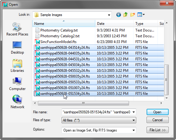
Opening an Image Set
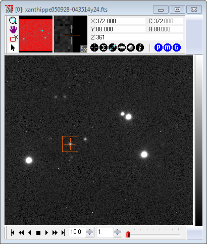
Now we will open an image set using a group of images of the field of minor planet Xanthippe provides with the Mira sample images. Let's do it: Open the File > Open dialog and select the xanthippe FITS images as shown at left, below. To do this, select the first image, then use Shift+click to mark a range of files (or Ctrl+click to mark individual files). Now look at the Options drop box at the bottom of the dialog. Make sure "Open as Image Set" is checked. If it is, all marked images are opened into 1 window. If not checked, then all marked images are opened into separate windows. Now click [Open] and watch all marked images open into a single Image Windows as shown at right, below.
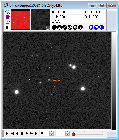
Using the controls on the Animation Toolbar at the bottom
of the Image Windows, you can select a particular image or animate the
entire image set. For example, click
![]() on the
Animation Toolbar. The default settings are for 10.0 frames per second and
every 1 image. After clicking this button, you should see the image set
animate. Notice a pattern of white dots that move toward the upper right
during animation. This set of image has been registered (aligned), and these
dots are hot pixels that were not corrected by the software used to
calibrate the images (not Mira). To see them better, you may need to change
the palette or transfer function or zoom or pan the images
— even while animation is running. Do it now:
Mouse down on the Colormap and move the mouse as described
above, or open the Palette Manager and change the palette.
After you have had some fun with this feature, stop the animation.
on the
Animation Toolbar. The default settings are for 10.0 frames per second and
every 1 image. After clicking this button, you should see the image set
animate. Notice a pattern of white dots that move toward the upper right
during animation. This set of image has been registered (aligned), and these
dots are hot pixels that were not corrected by the software used to
calibrate the images (not Mira). To see them better, you may need to change
the palette or transfer function or zoom or pan the images
— even while animation is running. Do it now:
Mouse down on the Colormap and move the mouse as described
above, or open the Palette Manager and change the palette.
After you have had some fun with this feature, stop the animation.
Measuring an Image Set
To show one measurement on the image set, move the
Image Cursor onto the star shown at left, below (after
this, do not move the Image Cursor for the next few
exercises). The cursor does not have to be centered before making the
measurement, but it should be within a couple of pixels of the center of the
star. Now click
![]() to
calculate the centroids. They open into a Report Window as
shown at right, below.
to
calculate the centroids. They open into a Report Window as
shown at right, below.
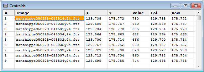
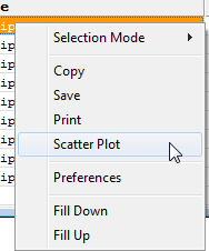
The columns labeled "X" and "Y" list world coordinates if the image(s) have a world coordinate calibration such as (RA, Dec) or mm. These images are not calibrated, so X and Y list Column and Row coordinates. How much do these measurements differ? One way to estimate this is to click the column header to sort the table. Click the Y column heading to sort the value from highest to lowest or lowest to highest value. After sorting values, you can return the table to its original measurement order by clicking the # column heading. Another option to view measurement data is to create a scatter plot. Here we will make a plot of Y coordinate versus image number. To do this, right click inside the Report window to open the menu as shown below, and select Scatter Plot. In the Scatter Plot dialog, select the columns you want to plot against each other. As shown at center, below, select # for the X-axis and Y for the Y-axis and click [Plot]. This creates the Plot window shown at right, below.
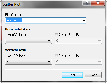
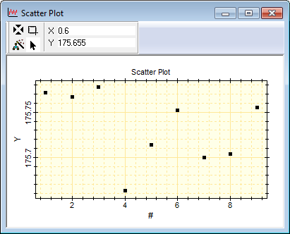
By roaming the crosshair around he Plot Window, you can easily determine the highest and lowest points differ by about 0.113 pixels. This is the maximum range and there appears to be no correlation between the centroid Y position and the image's index in its sequence. You can make all sorts of measurements and analyses just like this by using different commands available in Mira. These include distances and angles, statistics, centroids, aperture photometry, FWHM, and more.
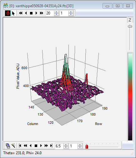
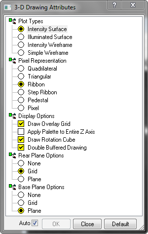
Creating a 3-D Plot Series
Plots (or "graphs") also can be made for the entire image
set by using the same commands as described above. In this case, let's make
a 3-D plot of all 9 images. Click the
![]() button to
create a 3-D Plot Window. After creating the plot, various
aspects of the plot can be changed to change the view, even while you
animating the 3-D plot set. The 3-D plot shown below was produced using the
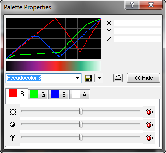
settings shown in the 3-D Drawing Attributes and
Palette Manager windows shown below.
button to
create a 3-D Plot Window. After creating the plot, various
aspects of the plot can be changed to change the view, even while you
animating the 3-D plot set. The 3-D plot shown below was produced using the
settings shown in the 3-D Drawing Attributes and
Palette Manager windows shown below.
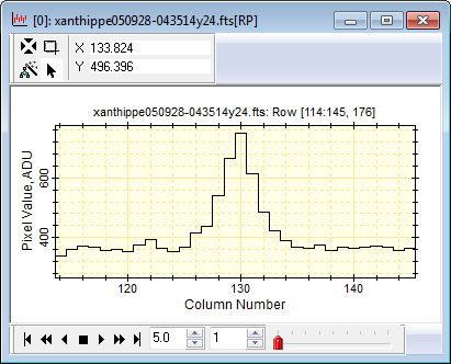
Finally, let us plot the row through the center of the
star where we moved the Image Cursor a few exercises ago.
To do this, click the Row Profile button
![]() on the
Main Toolbar. Right click on the plot and switch the Plot Series
Mode between Overplot and Animate
to produce the Plot Windows shown below. Notice that, in Animate
mode, the Plot Animation Toolbar opens in the Plot
Window just as for Image Windows and 3-D
Plot Windows.
on the
Main Toolbar. Right click on the plot and switch the Plot Series
Mode between Overplot and Animate
to produce the Plot Windows shown below. Notice that, in Animate
mode, the Plot Animation Toolbar opens in the Plot
Window just as for Image Windows and 3-D
Plot Windows.
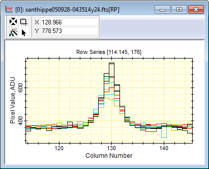
You can change the various plot series to have a single color using the Plot Series Attributes command described above (select a color or other attribute and then use the "copy down" menu command — see the User's Guide for details). You might also use the Plot Series Attributes dialog to highlight 1 or more specific plot series with a different color or a thicker line to see how it compares with the same plot from the other images.
Using Copy + Paste between Plot Windows
Finally, we will show how Mira's copy+paste command works
between Plot Windows. It also works between Image Windows, Editor Windows,
and Script Windows. In this example, we want to compare the radial profile
of 3 stars by plotting them on the same graph. Let's do it: Using the
Xanthippe image, move the Image Cursor onto one of the bright stars and
click
![]() to create a radial profile plot. We will call this first plot, "Plot 1". Now
move the cursor onto another bright star and create "Plot 2". With Plot 2 on
top, press Ctrl+C (or "Edit > Copy") to copy its contents.
Make Plot 1 the top-most window and press Ctrl+V (or "Edit
> Paste"). This pastes Plot 2 into the window of plot 1. Repeat this
procedure for the 3rd bright star, giving you 3 radial profile plots in the
window for Plot 1. It Plot 1 is not already in Overplot
mode, showing all 3 plots, right click on it and select "Plot Series Mode >
Overplot". The first plot and the final plot are shown below.
to create a radial profile plot. We will call this first plot, "Plot 1". Now
move the cursor onto another bright star and create "Plot 2". With Plot 2 on
top, press Ctrl+C (or "Edit > Copy") to copy its contents.
Make Plot 1 the top-most window and press Ctrl+V (or "Edit
> Paste"). This pastes Plot 2 into the window of plot 1. Repeat this
procedure for the 3rd bright star, giving you 3 radial profile plots in the
window for Plot 1. It Plot 1 is not already in Overplot
mode, showing all 3 plots, right click on it and select "Plot Series Mode >
Overplot". The first plot and the final plot are shown below.

If you wish to change the label titles and plot caption of "Plot 1" (or any plot), right click on the plot and select "Plot Attributes", then select the "Labels" tab.
This marks the end of the Tutorial. Numerous other tutorials are given in the Mira User's Guide.
Glossary of Terms
Understanding the terminology we use in this document will make it easier to learn Mira. The sections below define what is meant when the instructions tell you to drag the mouse or to be sure a window has focus.
Mouse Terminology
|
Click |
The action of pressing, then releasing the mouse button. Usually you do this to execute a command like that associated with a button, checkbox, or other control. |
|
Drag |
The action of moving the mouse while holding down the primary mouse button. During a drag operation, something will be moving or adjusting such as an image being centered or a line vector being stretched. |
|
Mouse Cursor |
The normal mouse pointer when it moves into an Image Window. The Image Window displays image coordinates and value as the pointer is moved over the image. This differentiates it from the Image Cursor, which marks reference positions on the image but does not give continuous updating of the image coordinate. |
|
Mouse Down |
The action of pressing the "primary" mouse button (normally the left button). Usually the mouse is held down to drag some user interface object. Many procedures in Mira require you to press and hold the mouse button while you move the mouse. |
|
Mouse Up |
The action of releasing the primary mouse button after some operation such as "dragging". |
|
Right Click |
The action of clicking the secondary mouse button, which is normally the right button. This is used to open Context Menus and for only a few other purposes. |
Window Terminology
|
Accelerator |
A keystroke combination that performs an operation that otherwise requires multiple keystrokes or mouse clicks. The accelerator would be a special key, like Ctrl+O for opening a file. |
|
Context Menu |
A popup menu that appears inside a view window by right clicking inside the window. In Mira, most View Windows have Context Menus. These open by right clicking inside the window you are working with. The name "Context Menu" derives from the fact that you do not lose your context (i.e., your train of thought) by right clicking where you are looking, as opposed to moving out of the window to hunt for a command in a menu somewhere else. |
|
Dialog Window (or Dialog) |
A type of window that is used to interact (i.e., to have a dialog) with the software. A Dialog doesn't usually show you any data or results. Images, plots, measurements, and other types of data or results are shown in View windows. Some dialogs take control of Mira and require you to click OK, Cancel, or Close before you can proceed. Others allow you to work with other windows while they are open. However, in both cases, a Dialog Window stays on top. |
|
Drop Dialog |
A dialog window that can expand downward to expose additional controls and information. These dialogs help you save screen space when you don't need to see everything. |
|
Focus |
Refers to a window that accepts input from the mouse or keyboard. When a window has focus, information about what you type or where you click the mouse is sent to that window. Usually, the window having focus is in front of other windows. |
|
Menu bar |
A menu containing pull down menus. The standard menu bars are located at the top of the Mira application window. Click the menu item on the menu bar to drop, or "pull down" a menu from the bar. Each type of View Window (Image, Plot, Report, Text Editor, and others) load their own specific menu bar containing commands appropriate for their type of control. |
|
Modal Dialog |
A window that takes control of the user interface. When a modal dialog is open in Mira, you cannot interact with any part of Mira outside that dialog. |
|
Modeless Dialog |
A Dialog Window that allows you to use other windows while open. |
|
Preference |
A parameter or setting that controls some aspect of the software. A number, a checkbox, a selection from a list — these are all "preferences". Usually preferences are displayed in a Dialog Window and changed by using dialog controls. |
|
Toolbar |
A row or column of buttons connected to commands, or software "tools". A toolbar attaches itself to the border of a window, usually along the top or left edge. Most toolbars may be detached from their parent window by dragging them after grabbing an area outside of the buttons. |
|
View Window |
A type of window that displays data, such as an image, plot, a table of measurements, or text. Usually a view window can be resized to give you a larger or smaller view of the data. |
Product Support & Information
|
|
|
|
World Wide Web |
|
|
Telephone |
+1.520.323.8600 (USA) |