Creating Plots from Images
This tutorial shows how to create some luminance plots from an image. Here we will make Line Profile Plots and Row Profile Plots from one of the sample images. See Plotting Commands for information about additional plot types and commands.
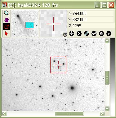
To create a plot, we need to first display an image (see Displaying Your First Image). After starting Mira, click the File > Open command in the main Menubar. This opens the normal the Open dialog. In this dialog, navigate to the 'Sample Data' subdirectory in the Mira installation folder and then open the image named 'hyak0324.120.fts'. The displayed image will look like the one shown below. Note that the image may appear larger or smaller than shown here, depending upon how Mira scales it to fit the screen.
Now magnify and re-center the image so that it looks like
the figure below. Next, open the Line Profile Toolbar by clicking ![]() on the main Image Plot Toolbar. The Line Profile Toolbar
opens on the left side of the Image Window as shown below.
on the main Image Plot Toolbar. The Line Profile Toolbar
opens on the left side of the Image Window as shown below.
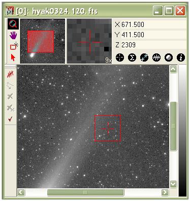
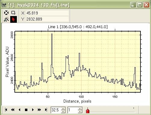
A Line Profile Plot shows the change in luminance
along a line drawn on the image. This type of plot uses the
Line Profile Toolbar
shown on the left side of the Image Window in the figure above.
This is a standard Command Toolbar which was opened by clicking
![]() on the Image Plot Toolbar at the top of the Mira
application window. This toolbar opened in the typical mode with
the top button (the marking mode) enabled. Using these toolbar
buttons you can plot the luminance along any vector drawn on the
plot and, as with other Mira plots, it works for both RGB images
and non RGB images. To make a plot, mouse simply down at the
starting point, then drag the line to its ending point and release
the mouse. You will get a plot that looks like this:
on the Image Plot Toolbar at the top of the Mira
application window. This toolbar opened in the typical mode with
the top button (the marking mode) enabled. Using these toolbar
buttons you can plot the luminance along any vector drawn on the
plot and, as with other Mira plots, it works for both RGB images
and non RGB images. To make a plot, mouse simply down at the
starting point, then drag the line to its ending point and release
the mouse. You will get a plot that looks like this:
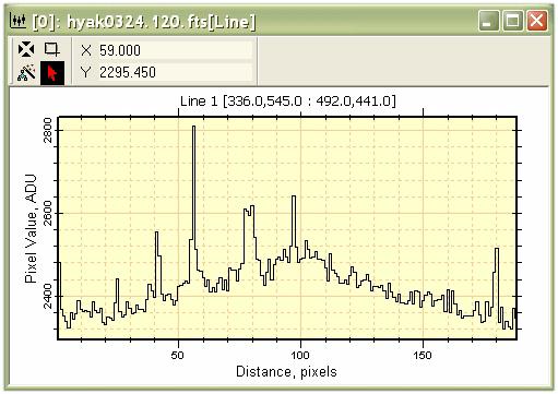
Next we want to know what is happening to pixels along a parallel line beside the one we just drew on the image. Click the second button on the toolbar to enter Move Mode for the marker (the line). Next, point at the line and click the mouse down to grab it and then drag the line to a new location as described in Move perpendicular. When the mouse is released, the next profile over-plots the first one, like so:
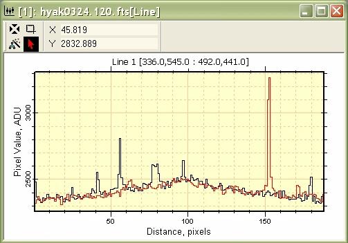
We can continue adding plot series forever. But at
some point we will want to change to another mode, or click
![]() to return to the default Roam Mode.
If you don't like the appearance of the Plot Window, press
Ctrl+A to open the Plot Attributes
dialog.
to return to the default Roam Mode.
If you don't like the appearance of the Plot Window, press
Ctrl+A to open the Plot Attributes
dialog.
When more than 1 plot series exists, you can choose to over-plot or animate them 1 series at a time. Right click on the plot to open the Plot Context Menu and select Plot Series Mode > Animate (you can also get this command from the Plot menu when an Image window has the focus) This command changes the window appearance to:
The Plot Animation Toolbar allows you to step or animate through the stack. Notice that you now see only 1 series at a time in Animate mode. You can switch back to Over-Plot in the same way.
Using Over-Plot and Animate modes in a Plot Window is a parallel to what can be done in an Image Window using Mira's unique concepts of Image Sets and File Lists, which are covered in another Tutorial.
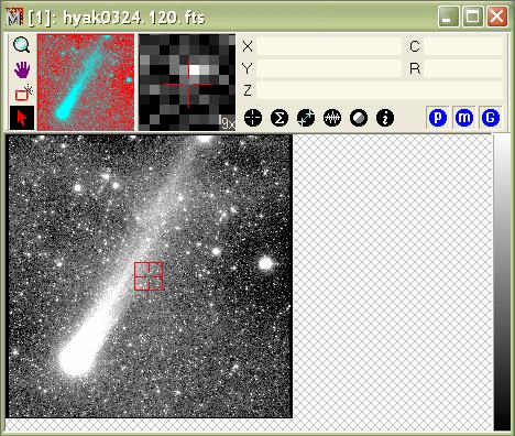
Next, let us plot the profile of a single row through the peak of a star. To make a Column Profile Plot or Row Profile Plot, we use the Image Cursor to mark the extent of the plot. To plot a Row Profile, you must first adjust the Image Cursor to enclose the columns and rows you want to use. Often we would do that by moving and sizing the Image Cursor. In this case we may want to set the length of the plot (the number of columns) and we want to position it on the peak of a star. There are several ways to position the Image Cursor on the peak:
One way is to have a steady hand and carefully position the image cursor using by microscopic mouse movements while watch for the peak pixel value to appear in the Image Coordinate Display box at the top of the Image Window. This may not give you what you want if the image is de-magnified because not every pixel can be hit by mouse movements. And there are easier ways.
Another method is to magnify the image so it is easier to position the mouse on the center of the star. You can use the mouse to position the Image Cursor or, if the window has focus, you can position it using the keyboard arrow keys. The window does have focus if you have clicked on it.
Still another method is to crudely position the
Image Cursor within a few image pixels of the peak. Then click
![]() on the Image Toolbar to home the
Image Cursor to the centroid position near where you dropped it
with the mouse.
on the Image Toolbar to home the
Image Cursor to the centroid position near where you dropped it
with the mouse.
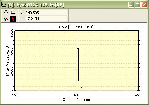
Now that the Image cursor is positioned on a star,
click ![]() to plot the single row at
the center of the Image Cursor. This button executes the Row
Profile Plot command. Clearly Method 3, above, is the quickest way
to get a row profile plot through the center of a star. And it
shows why some commands such as Centroid, Statistics, and Profile Plots are all linked to
the Image Cursor. Notice that the plot caption (not the window
caption) reminds us of the columns and rows we just plotted. In
this case, [350:450, 848] tells
us that we plotted from column 350 to 450 along row 848. Since we
centroided before making the plot, the center of the plot passes
through the peak of the star profile.
to plot the single row at
the center of the Image Cursor. This button executes the Row
Profile Plot command. Clearly Method 3, above, is the quickest way
to get a row profile plot through the center of a star. And it
shows why some commands such as Centroid, Statistics, and Profile Plots are all linked to
the Image Cursor. Notice that the plot caption (not the window
caption) reminds us of the columns and rows we just plotted. In
this case, [350:450, 848] tells
us that we plotted from column 350 to 450 along row 848. Since we
centroided before making the plot, the center of the plot passes
through the peak of the star profile.
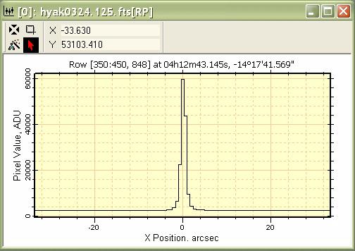
The plot above may have appeared differently if we
were plotting in units of World Coordinates. if the image has a World
Coordinate System calibration, with Right Ascension and Declination
for every point, then you can choose to plot in those coordinates.
The choice is specified a number of places in Mira, one being in
the Image Context Menu > Plot menu. Right click on the
image to open the Image Context Menu, select the Plot submenu,
then the check the World Coordinate
item. Then click ![]() again, and a plot
is created like the one below with World Coordinate position on the
X axis. Roaming the mouse pointer around either plot lists the
coordinates in whichever Plot Coordinate System was used.
again, and a plot
is created like the one below with World Coordinate position on the
X axis. Roaming the mouse pointer around either plot lists the
coordinates in whichever Plot Coordinate System was used.
To make the plot below, we used the image 'hyak0324.125.fts', which is a sample image having a World Coordinate System calibration pre-applied (note: the calibration is not correct but is included simply to show how World Coordinates are used).
The tutorial Displaying Your First Image Set shows how to over-plot the row profiles for members of an image set.
The previous sections have described how to over-plot multiple line profiles by using Move mode for the Line Profile Plot.
1. Make sure the window containing the image is the window with focus (it shows the highlighted caption).
2. Change the Image Cursor to a rectangle and
adjust the size to approximately 51 rows tall by 51 columns wide,
as shown below. The width may be any number, but this was the
default
image cursor size when the window opened. In Image Cursor Mode
(![]() button), move the cursor to pixel
(720,534) as shown below.
button), move the cursor to pixel
(720,534) as shown below.
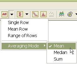
On the Image Plot Toolbar, click the down arrow next to the Row Profile command and select Averaging Mode > Mean as shown below.
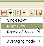
Using the Row Profile down arrow, execute the Mean Row command as shown below.
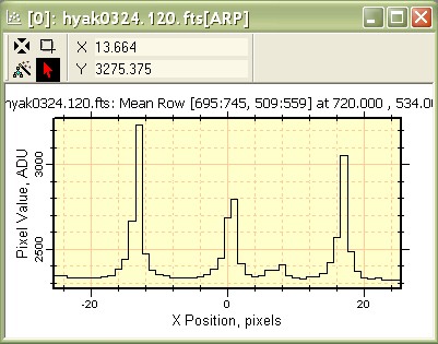
This creates a Mean row plot over 51 rows, as shown below.
Getting Started, Displaying Your First Image Set, Plotting Commands