Open this dialog from the "Create Synthetic
Image" command on the Process menu or by clicking the
![]() button on the main
toolbar.
button on the main
toolbar.
Create Synthetic Image
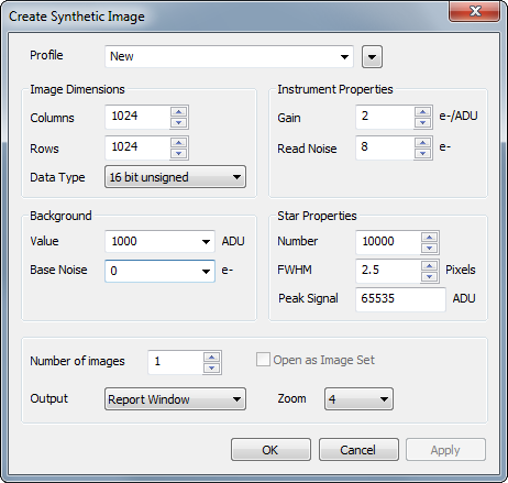
The Create Synthetic Image command creates realistic images containing noise and optionally, stars. These images are essential for evaluating processing and measurement algorithms and exploring the effects of noise and noise propagation through calibration strategies.
The noise model used for creating the synthetic image includes all forms of noise. Optionally, a realistic distribution of randomly placed stars may be added with a Gaussian point spread function ("PSF"). All parameters are specified in commonly used units of electrons (e-) and DN (or ADU's).
Open this dialog from the "Create Synthetic
Image" command on the Process menu or by clicking the
![]() button on the main
toolbar.
button on the main
toolbar.
|
Profile |
Selects a parameter collection for display in the dialog. |
|
Columns |
The number of columns in the new image. |
|
Rows |
The number of rows in the new image. |
|
Data Type |
Select the data type of the new image. |
|
Gain |
The electronic gain of the camera system, in units of electrons per number (also called e/ADU). |
|
Read Noise |
The camera readout noise in units of electrons. |
|
Value |
The background value of the image. This is specified in units of DN (digital numbers). The DN value is related to the number of electrons using the Gain. |
|
Base Noise |
The base level of noise measured in units of electrons. This is a supplemental, additive noise term, and usually would be set to 0. The camera readout noise is entered as a separate parameter. |
|
Number |
The number of stars to create. A consequence of the stellar luminosity function is that most stars will be very faint. |
|
FWHM |
The Full Width at Half Maximum ("FWHM") brightness, measured in units of pixels. Note: This describes a diameter, not a radius. |
|
Peak Signal |
The maximum signal used for creating stars. In combination with the Data type and Value parameters, it is possible to set this value such that the brightest stars may be saturated above the counting limit of the data type. For example, using Data type = "16 bit unsigned", Value=10000, and Peak Signal = 65000 will allow the brightest star to peak around 75000 DN, which is above the 65535 DN limit of 16-bit data. |
|
Number of images |
This specifies the number of independent images to create using the parameter set. If more than 1, the Open as Image Set check box appears. |
|
Results |
Specifies the output location for listing the properties of the synthetic stars that are created. The options are None (no data are listed), a Mira Text Editor window, and a Mira Report window. Saving the results to a Report window provides added benefits, including the ability to perform analyses on the grid data and to send the image cursor to any star location to identify it on the image (see below). |
|
Open as Image Set |
If Number of images > 1, this specifies whether the images are opened in separate windows or as an image set in a single window. |
Schematically, the image value at any pixel location is given as follows:
|
|
Image value = (Background Value + PSF Values + Noise) / Gain. |
where the Noise value is a Gaussian random value and may be positive or negative. The PSF value is the sum of all stellar PSF's evaluated at the gicen pixel location. All values are used in fundamental units of electrons (or photons) and then converted to pixel value in units of DN (Digital numbers, or ADU) as would be recorded in an image. As per convention in the field of scientific imaging, some parameters are entered using fundamental units while others are entered using ADU (or DN) units; the units are indicated on the Create Synthetic Image dialog.
The Noise value above is computed from all sources of which all are assumed to be uncorrelated. The noise can be described as follows:
|
|
Noise squared = Sum of Squares of (Background Noise, PSF Shot Noise, Base Noise, Readout Noise, Digitization Noise) |
Notice that some of the noise terms are a function of the signal while others are constant. Of those that depend on the signal, Background noise is the "shot noise" of the background signal and PSF shot noise is the photon noise for all PSF's that overlap a given pixel location. All noise sources are computed in fundamental units of electrons (or, equivalently, photons).
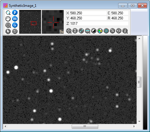
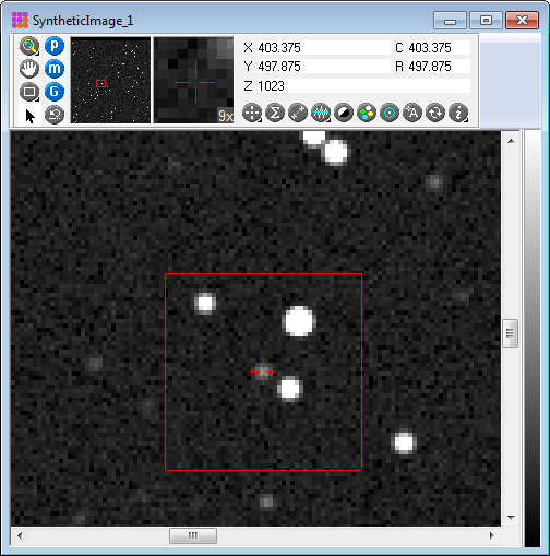
The following example illustrates the process of creating and analyzing a synthetic star field. The image below shows a portion of the synthetic image produced using the parameters shown in the dialog above. This example created 10,000 artificial stars, most of which are faint because of the stellar luminosity function.
Data for the 10,000 artificial stars were listed in the Report window shown below. The listed intensity is not the peak value but, rather, gives the total volume under the Point Spread Function ("PSF"). This intensity is the target value for which the PSF was created, and hence it is a "pre noise" value. The actual intensity measured for any artificial star will differ because of random noise sources included in the model.
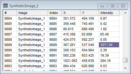
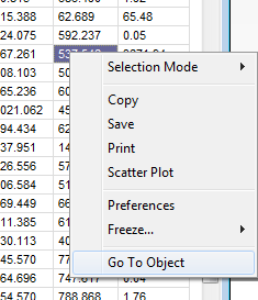
The Report window includes a pop-up menu which is opened by right-clicking the mouse, as shown below. After selecting (highlighting) the target star, the "Go to Object" command was clicked to center the image cursor on star 9889 as shown in the Report. The centered star is shown in the image window below.
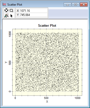
In the next picture, the Scatter Plot command was selected from the menu. If the positions of the artificial stars are random, then there should be no correlation between x and y coordinates. To investigate this, the scatter plot below was created from the tabular star data. After the plot was created, the Plot Series Attributes command was used to change the default squares to smaller dots:
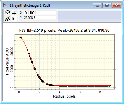
The following window shows a radial profile plot for one a medium-bright artificial stars. The calculated FWHM is 2.519, identical within the noise to the target FWHM value of 2.5. Remember that noise in the synthetic image results in measured quantities scattering about their known target value.
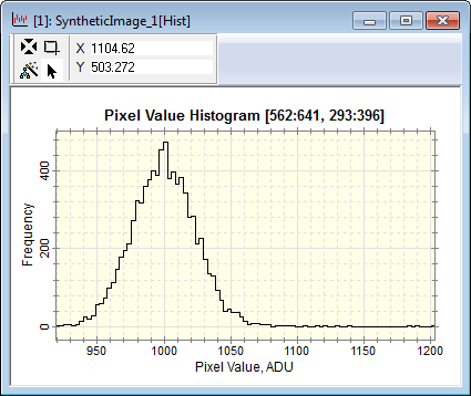
Another test shows the histogram of a region of "sky" background. The image region outlined below was sampled to produce the histogram plot following.
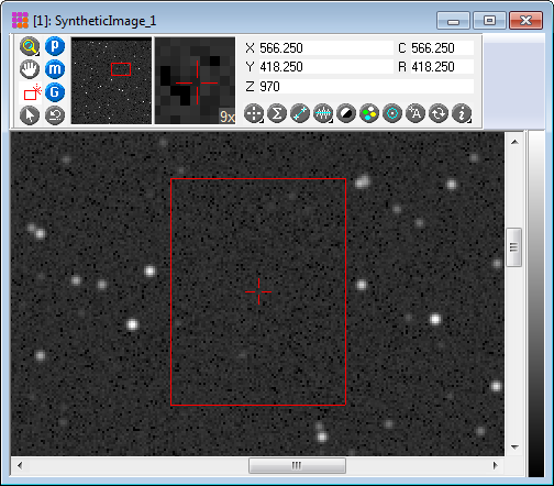
As shown below, the longer positive tail in the histogram results from the many, extremely faint stars present inside the sampling rectangle. Note that the sky histogram has a Gaussian shape because of the Gaussian random noise in the model and is centered on 1000 as specified in the parameter dialog.