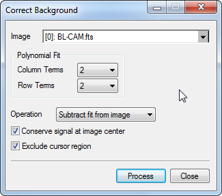
Correct Background
The Correct Background command computes a polynomial fit to an image surface and applies the fit to the image. The fit may be subtracted from the image or divided into the image to flatten the image background. You also can choose to store the fit surface in the image data if you want to save the surface as a separate image.
Open this dialog from the Process > Math menu.
Parameters of the Correct Background Command
|
Image |
Select the image or image set to process from the drop list. |
|
Column Terms |
Select the number of polynomial terms to fit data in the horizontal direction. |
|
Row Terms |
Select the number of polynomial terms to fit data in the vertical direction. |
|
Operation |
Choose the operation you want to apply: Subtract Fit: The surface fit is subtracted from the image. The removes additive effects, like scattered light. Divide Fit: The surface fit is divided into every pixel of each image. Mira automatically converts the output image(s) to a real data type to handle the non integral luminance values that result from the division. This corrects multiplicative effects, like vignetting or sensitivity. Replace Fit: The surface fit is replaced into the image array. |
|
Conserve signal at image center |
Check this box if you want the resulting image to have a similar signal level before and after subtracting or dividing the fit. Otherwise the result will end up with a typical signal near zero after subtracting the fit, or near 1 after dividing the fit. |
|
Exclude cursor region |
When computing the surface fit, this command can be instructed to ignore a rectangular region of pixels. The region is defined by the Image cursor, so the image cursor should be adjusted to outline the exclusion region before clicking OK to execute the command. |
This command calculates and (optionally) corrects either an additive effect, like scattered light, or a multiplicative effect, like vignetting, by fitting and applying a polynomial surface to the image. The polynomial ranges from 1x1 to 10x10 (100 terms). Clearly, 1x1 represents a constant value, but 1x2 and 2x1 represent a slope parallel to 1 axis. A 2x2 polynomial models a warped plane. A 3x3 fit involves a paraboloid and often is a good starting point for correcting calibrated images that appear to show poorly corrected vignetting which results from the optical axis shifting relative to the flat field images.
In general you should use the lowest order that adequately flattens the background. The quality of the correction can be assessed by carefully examining the image at high contrast or after adjusting the palette, by making a contour plot, or by evaluating horizontal and vertical cross sectional plots at various places on the image (see the example, below).
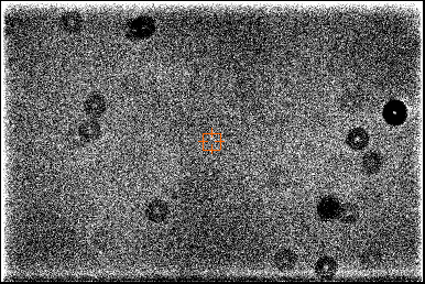
The following example shows the power of this command by correcting an extreme example of background curvature. The "before" image below shows a flat field frame, which was selected because it had a large amount of background curvature:
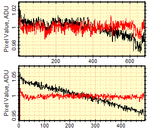
Below are shown cross sectional plots which illustrate the degree of non-flatness in the image. Black curves show the original image, red shows the corrected image. The small dips in the upper curves are caused by dust shadows on the flat field image and are not related to the background curvature. The data were over-plotted using the Plot Series Attributes command and the Copy+Paste capability of Plot windows.
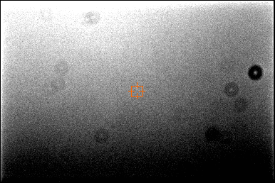
The "after" image below shows the result of correcting the background using the Conserve signal as image center option. In this view, the palette was stretched to high contrast for close evaluation of the image flatness. Notice that the deviations from flatness are now significantly below the noise level over all but the extreme edges of the image.