Tutorial: Doing Time Series Photometry
This tutorial describes how to use the Aperture Photometry package to do time series photometry on a set iof images of the minor planet Xanthippe. In this tutorial we use observations of the minor planet Xanthippe to place limits on variations in its brightness over a short time period. In minor planet studies, these variations are used to characterize the rotation or tumbling of the body. The same methods could be used for analysis of variable stars, to search for stellar eclipses caused by extra-solar planets orbiting stars, or for other types of investigation.
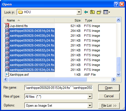
We begin by opening an image set containing 9 calibrated images of the minor planet Xanthippe. First, click File > Open on the main menu to open the Open dialog. Now click on the first image of the image set, hold down the [Shift] key, and mark the last image of the image set to highlight all 9 target images as shown below (see Opening Multiple Images).
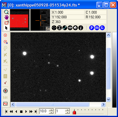
Make sure the Open as Image Set option is checked at the bottom of the Open dialog, then click [Open] to open the images. They appear in an Image Window like this:
Next, click the ![]() on the
main toolbar to open the aperture photometry package and its
toolbar. On the toolbar, click
on the
main toolbar to open the aperture photometry package and its
toolbar. On the toolbar, click ![]() to open
the Aperture tool
window for setting the aperture parameters. After setting the radii
and other parameters to the desired values, close the Aperture tool
window. Here we used circular apertures with radii of 4, 13, and 23
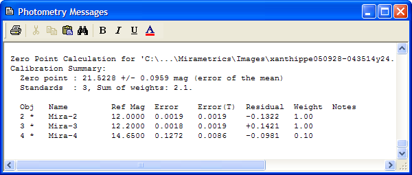
pixels. These values are listed at the beginning of the results in
the Photometry Messages window (see below).
to open
the Aperture tool
window for setting the aperture parameters. After setting the radii
and other parameters to the desired values, close the Aperture tool
window. Here we used circular apertures with radii of 4, 13, and 23
pixels. These values are listed at the beginning of the results in
the Photometry Messages window (see below).
On the aperture photometry toolbar click ![]() to select Target
Mode and mark the target object on the first image. Also,
mark a check star to be used to monitor the stability of the
photometry from image to image. Then click
to select Target
Mode and mark the target object on the first image. Also,
mark a check star to be used to monitor the stability of the
photometry from image to image. Then click ![]() to select Standard Mode and mark the 3 standards on the
first image. Each time a standard is marked, you will need to enter
its magnitude (and possibly other, optional information) into the
Standard
Data dialog as shown below.
to select Standard Mode and mark the 3 standards on the
first image. Each time a standard is marked, you will need to enter
its magnitude (and possibly other, optional information) into the
Standard
Data dialog as shown below.
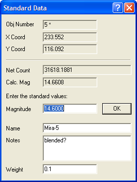
In the Standard Data dialog we also added a comment for this object and changed its weight to 0.1 of that used for the other standard stars. The minor planet moves close to this star in the last 4 or 5 images, hence the profiles may be blended. We also could use the Star Removal package to remove this star from the image before doing the aperture photometry. This is discussed further at the end of this tutorial.
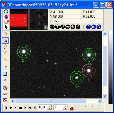
The Image Window now should show 4 objects as shown below. Object 1 is the minor planet Xanthippe.
Next we want to extend the marked objects from
image 1 to all images in the image set. To do this, click ![]() on the toolbar. Next, calculate everything by
clicking
on the toolbar. Next, calculate everything by
clicking ![]() . This produces a verbose
listing of the standard star measurements and the photometric zero
point calculations in a Text Editor window. The picture below shows the
results for the 9-th image.
. This produces a verbose
listing of the standard star measurements and the photometric zero
point calculations in a Text Editor window. The picture below shows the
results for the 9-th image.
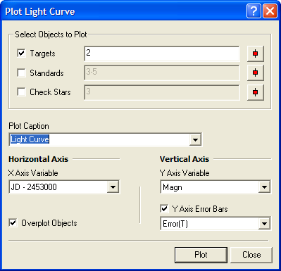
Next we will plot a light curve from these
observations. On the Aperture Photometry toolbar click ![]() to open the Plot Light Curve dialog.
In the Targets field, enter the number
1 so that object 1 is plotted. Uncheck the Standards and Check
Stars boxes so that the plot will auto-scale to only the
minor planet we measured. These observations were made over the
course of a night so we could make a plot using "Time (Hours)" or
"Time (Minutes)" on the Horizontal
Axis. Instead, we will select "JD - 2453000" from the drop
down list. The JD option takes its name from the column title in
the Photometry Measurements table. A Julian Date Offset
of 2453000 was entered on the Other
Preferences page before the photometry was done.
to open the Plot Light Curve dialog.
In the Targets field, enter the number
1 so that object 1 is plotted. Uncheck the Standards and Check
Stars boxes so that the plot will auto-scale to only the
minor planet we measured. These observations were made over the
course of a night so we could make a plot using "Time (Hours)" or
"Time (Minutes)" on the Horizontal
Axis. Instead, we will select "JD - 2453000" from the drop
down list. The JD option takes its name from the column title in
the Photometry Measurements table. A Julian Date Offset
of 2453000 was entered on the Other
Preferences page before the photometry was done.
Click [Plot] on the Plot Light Curve dialog to produce the following plot containing magnitude error bars:
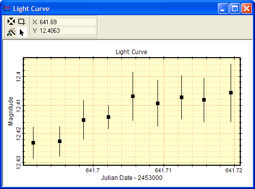
The error bars here are relatively large because the standard star magnitudes we entered were not nearly as precise as the actual uncertainties of the measurements. Therefore, the uncertainty in the calculated photometric zero point dominates the uncertainty in the measurements of the target object, Xanthippe. You can see this effect by inspecting the standard star data listed in the Photometry Messages text window (see above). For image 9, the zero point value is listed as 21.4819 +/- 0.0049. This value combines the scatter in the standard star magnitudes (see the Residuals column) and also the "random" error for each standard star measurement itself. The random error for each standard star is listed in the Error and Error(T) columns. Notice that the star "Mira-4", which is object 4, has a large random error that is caused by becoming progressively more blended with Xanthippe starting around image 5 of the image set. We set its weight to 0.1, so that object 4 would have only a small effect on the photometric zero points.
What do we do about the interference between object
4 and the image of Xanthippe in the last 5 images? First, we should
not have used object 4 as a standard star. Looking at the light
curve, you can see that the magnitude of Xanthippe increases
through the image set, especially in the last 5 images. Is this an
artifact of the blending? This could be verified by using the
Star Removal package
to remove object 4 from all images before doing the photometry.
Since the objects are already marked and their data are already
entered, this is not difficult to do. First, click ![]() on the Aperture Photometry toolbar and then
delete the marker for object 4 in image 1. Track this through the
image set. Then open the Star Removal package and remove object 5 from all
images. finally, using the Aperture Photometry toolbar again, track
the markers through the image set and click
on the Aperture Photometry toolbar and then
delete the marker for object 4 in image 1. Track this through the
image set. Then open the Star Removal package and remove object 5 from all
images. finally, using the Aperture Photometry toolbar again, track
the markers through the image set and click ![]() to re-calculate all the the zero point
calibrations and magnitudes for the target objects.
to re-calculate all the the zero point
calibrations and magnitudes for the target objects.
Contents, Tutorials, Aperture Photometry Preferences, Tutorial: Introduction to Aperture Photometry, Import Photometry Catalog, Photometric Measurements, Aperture Tool, Report Windows, Photometry Keywords, Tutorial , Using Edit Mode in Aperture Photometry, Preparing an AAVSO Report, Plotting a Light Curve, Kwee - van Woerden Solver