Tutorial: Creating Plots from Images
This tutorial teaches you how to create luminance plots from images. In this exercise we will make Line Profile Plots and Row Profile Plots from one of the sample images. For further information about plotting, see Plotting Commands, Working with Plots, Plotting Examples, and Examples of Row Plots.
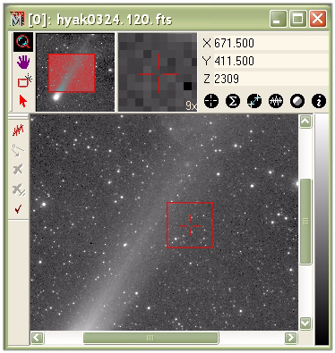
To create a plot, we need to first display an image (see Tutorial: Displaying an Image). After starting Mira , click the File > Open command in the main menu bar. This opens the normal the Open dialog. In this dialog, navigate to thr sample images in the folder "My Pictures\Mirametrics\Mira Pro 7 UE\Sample Data". Open the image named 'hyak0324.120.fts'. The displayed image will look like the one shown below. Note that the image may appear larger or smaller than shown here, depending upon how Mira scales it to fit the screen.
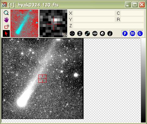
Now magnify and re-center the image so that it looks like the figure below. Next, open the Line Profile Toolbar by clicking on the main Image Plot Toolbar. The Line Profile Toolbar opens on the left side of the Image Window as shown below.
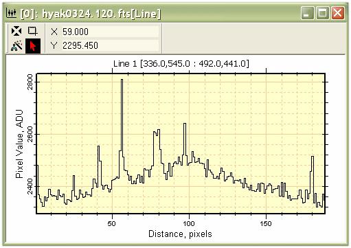
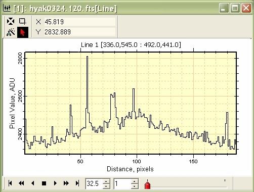
A Line Profile Plot shows the change in luminance along a line drawn on the image. This type of plot uses the Line Profile Toolbar shown on the left side of the Image Window in the figure above. This is a standard Command Toolbar which was opened by clicking on the Image Plot Toolbar at the top of the Mira application window. This toolbar opened in the typical mode with the top button (the marking mode) enabled. Using these toolbar buttons you can plot the luminance along any vector drawn on the plot and, as with other Mira plots, it works for both RGB images and non RGB images. To make a plot, mouse simply down at the starting point, then drag the line to its ending point and release the mouse. You will get a plot that looks like this:
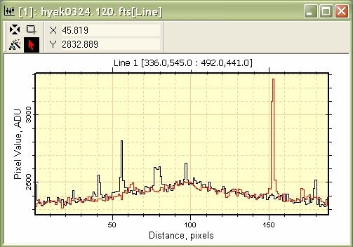
Next we want to know what is happening to pixels along a parallel line beside the one we just drew on the image. Click the second button on the toolbar to enter Move Mode for the marker (the line). Next, point at the line and click the mouse down to grab it and then drag the line to a new location as described in Move perpendicular. When the mouse is released, the next profile Overplots the first one, like so:
We can continue adding plot series forever. But at
some point we will want to change to another mode, or click
![]() to return to the default Roam Mode.
If you don't like the appearance of the Plot Window, press
Ctrl+A to open the Plot Attributes
dialog.
to return to the default Roam Mode.
If you don't like the appearance of the Plot Window, press
Ctrl+A to open the Plot Attributes
dialog.
When more than 1 plot series exists, you can choose to Overplot or animate them 1 series at a time. Right click on the plot to open the Plot Context Menu and select Plot Series Mode > Animate (you can also get this command from the Plot menu when an Image window has the focus) This command changes the window appearance to:
The Plot Animation Toolbar allows you to step or animate through the stack. Notice that you now see only 1 series at a time in Animate mode. You can switch back to Overplot in the same way.
Using Overplot and Animate modes in a Plot Window is a parallel to what can be done in an Image Window using Mira's unique concepts of Image Sets and File Lists; these are covered in another tutorial.
Next, let us plot the profile of a single row through the peak of a star. To make a Column Profile Plot or Row Profile Plot, we use the Image Cursor to mark the extent of the plot. To plot a Row Profile, you must first adjust the Image Cursor to enclose the columns and rows you want to use. Often we would do that by moving and sizing the Image Cursor. In this case we may want to set the length of the plot (the number of columns) and we want to position it on the peak of a star. There are several ways to position the Image Cursor on the peak:
One way is to have a steady hand and carefully position the image cursor using by microscopic mouse movements while watch for the peak pixel value to appear in the Image Coordinate Display box at the top of the Image Window. This may not give you what you want if the image is de-magnified because not every pixel can be hit by mouse movements. And there are easier ways.
Another method is to magnify the image so it is easier to position the mouse on the center of the star. You can use the mouse to position the Image Cursor or, if the window has focus, you can position it using the keyboard arrow keys. The window does have focus if you have clicked on it.
Still another method is to crudely position the
Image Cursor within a few image pixels of the peak. Then click
![]() on the Image Toolbar to home the Image Cursor to the
centroid position near where you dropped it with the mouse.
on the Image Toolbar to home the Image Cursor to the
centroid position near where you dropped it with the mouse.
Now that the Image cursor is positioned on a star,
click ![]() to plot the single row at the
center of the Image Cursor. This button executes the Row Profile
Plot command. Clearly Method 3, above, is the quickest way to get a
row profile plot through the center of a star. And it shows why
some commands such as Centroid, Statistics, and Profile Plots are all linked to
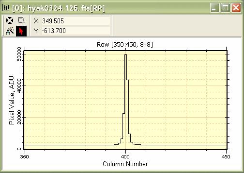
the Image Cursor. Notice that the plot caption (not the window
caption) reminds us of the columns and rows we just plotted. In
this case, [350:450, 848] tells
us that we plotted from column 350 to 450 along row 848. Since we
centroided before making the plot, the center of the plot passes
through the peak of the star profile.
to plot the single row at the
center of the Image Cursor. This button executes the Row Profile
Plot command. Clearly Method 3, above, is the quickest way to get a
row profile plot through the center of a star. And it shows why
some commands such as Centroid, Statistics, and Profile Plots are all linked to
the Image Cursor. Notice that the plot caption (not the window
caption) reminds us of the columns and rows we just plotted. In
this case, [350:450, 848] tells
us that we plotted from column 350 to 450 along row 848. Since we
centroided before making the plot, the center of the plot passes
through the peak of the star profile.
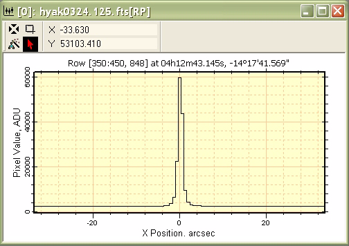
The plot above may have appeared differently if we
were plotting in units of World Coordinates. if the image has a World
Coordinate System calibration, with Right Ascension and Declination
for every point, then you can choose to plot in those coordinates.
The choice is specified a number of places in Mira , one being in
the Image Context Menu > Plot menu. Right click on the
image to open the Image Context Menu, select the Plot submenu,
then the check the World Coordinate
item. Then click ![]() again, and a plot
is created like the one below with World Coordinate position on the
X axis. Roaming the mouse pointer around either plot lists the
coordinates in whichever Plot Coordinate System was used.
again, and a plot
is created like the one below with World Coordinate position on the
X axis. Roaming the mouse pointer around either plot lists the
coordinates in whichever Plot Coordinate System was used.
To make the plot below, we used the image 'hyak0324.125.fts', which is a sample image having a World Coordinate System calibration pre-applied (note: the calibration is not correct but is included simply to show how World Coordinates are used).
The tutorial Tutorial: Displaying an Image Set shows how to Overplot the row profiles for members of an image set.
The previous sections have described how to Overplot multiple line profiles by using Move mode for the Line Profile Plot. Mira also lets you Overplot the plot data (series) from any Plot window onto the data displayed in any other Plot window. To do this, use the Copy/Paste protocol to copy the series from a "source" plot and paste them into a "destination" plot. For example, using the image 'Hyak0324.120.fts' from above, let us compare a median combination of about 20 rows with a mean combination of the same rows.
1. Make sure the window containing the image is the window with focus (it shows the highlighted caption).
2. Change the Image Cursor to a rectangle and
adjust the size to approximately 51 rows tall by 51 columns wide,
as shown below. The width may be any number, but this was the
default
image cursor size when the window opened. In Image Cursor Mode
(![]() button), move the cursor to
pixel (720,534) as shown below.
button), move the cursor to
pixel (720,534) as shown below.
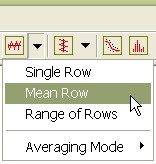
3. On the Image Plot Toolbar, click the down arrow next to the Row Profile command and select Averaging Mode > Mean as shown below.
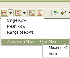
Using the Row Profile down arrow, execute the Mean Row command as shown below.
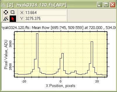
This creates a Mean row plot over 51 rows, as shown below.
5. Repeat the previous step using Averaging Mode > Median followed by the Median Row command to create the following plot. If the toolbar command is not available, click on the image to give it focus and load its toolbar. Note that the Averaging mode change applies to this image window only. To make a setting the default, see Plot Averaging Mode
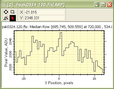
In the above plots, compare the Y-axis scales to see the difference between the median of 51 rows and the mean of 51 rows.
6. Click the Median Row Plot (the first one of the two we created) to activate it. Now click the Edit > Copy command in the Plot menu or use Ctrl+C to copy the data from the Median Row Plot window.
7. Click the Mean Row Plot window to activate it. Now click the Edit > Paste command in the Plot menu or use Ctrl+V to paste the data into the Mean Row Plot window. The result looks like the following:
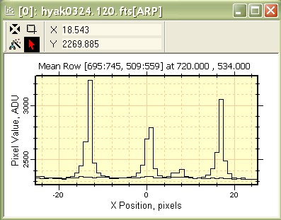
After you paste the data into the window as shown above, you might wish to open the Plot Animation Toolbar so you can blink between the plot series. You will also notice that the plot caption changes when you change the series.
You can access the plot data values directly using the Series Data command. With the last window active, right click on it to open the Plot Context menu, then select the Series Data command. This opens a window which looks like the following:
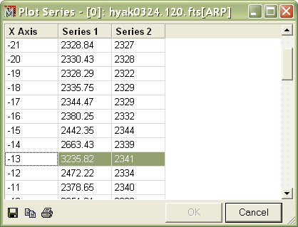
In the Plot Series dialog, the row at X Axis = -13 has been highlighted by dragging the mouse point across it to show a position where the mean and median row values are very different. You can also see this in the plot windows above. You can save the data from the Plot Series dialog using the buttons on its bottom border or by using commands in its context menu (right click on the table to open). See Working with Plot Series Data.
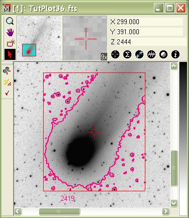
Mira provides two ways to plot contours on an image: 1) Contours computed at specific luminance levels, and 2) a single contour computed at a level you mark on the image. Here, we will mark a contour on the comet image we have been using thus far.
To interactively draw a contour, do the following:
Select the image 'Hyak0324.120.fts' (click on its window if it does not already have focus).
Outline a region of interest by positioning and sizing the Image Cursor. The contour will be computed inside this region.
Click the Interactive Contour command button ![]() on the main toolbar. This opens the Interactive Contour toolbar at the left margin
of the Image Window. The toolbar opens in marking mode. If you
leave marking mode, you can re-enter by clicking the top button on
the interactive contour plotting toolbar.
on the main toolbar. This opens the Interactive Contour toolbar at the left margin
of the Image Window. The toolbar opens in marking mode. If you
leave marking mode, you can re-enter by clicking the top button on
the interactive contour plotting toolbar.
Click the left mouse button on the luminance
level where you want to create the contour. To change the contour
smoothness or color, open the Interactive
Contour Preferences by clicking ![]() on the toolbar.
on the toolbar.
In the picture below, the contour was marked at a luminance value of of 2419. One way to enhance the information give by the contour is to switch to a pseudocolor palette and adjust it to appear dark near the luminance level of the contour but to show color above and below that value.
|
Note |
It is usually advisable to constrain the contour using as small a region as necessary by using the image cursor. Contours require drawing many short lines, and a complex contour containing a huge number of line segments may cause the computer to lag when redrawing the image window. |
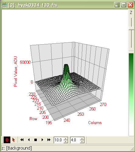
Mira can quickly create a 3-D Surface Plot showing the surface luminance versus (column,row) position in the image. Like contour plots, 3-D plots work with the region bounded by the Image Cursor and should be constrained to a small number of pixels, usually not more than 10,000 pixels in area unless the image is very noise-free. Otherwise, plotting many pixels often just shows a rough noise surface with little information. Various types of 3-D plots are available; see 3-D Pixel Representations to view some of these variations.
Select the image 'Hyak0324.120.fts' (click on its window if it does not already have focus).
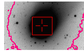 Outline a region of
interest by positioning and sizing the Image Cursor. The 3-D surface will be rendered
inside this region. Here, we moved the cursor to near the center of
the comet nucleus.
Outline a region of
interest by positioning and sizing the Image Cursor. The 3-D surface will be rendered
inside this region. Here, we moved the cursor to near the center of
the comet nucleus.
Click the 3-D Surface Plot command button ![]() on the Image Plot Toolbar.
on the Image Plot Toolbar.
To quickly reorient the plot to a different
viewpoint position, click ![]() on the Rotation Toolbar to
enter rotation mode. To rotate the image, mouse down inside the
plot window and hold down the button while you move the mouse to
move the plot viewpoint.
on the Rotation Toolbar to
enter rotation mode. To rotate the image, mouse down inside the
plot window and hold down the button while you move the mouse to
move the plot viewpoint.
The 3-D plot takes its palette from that used in the 2-D image. After the 3-D plot is drawn, you can change its appearance using the 3-D drawing attributes dialog and other tool windows. You can also adjust the palette to enhance the rendering as shown below.
Contents, Tutorials, Getting Started, Tutorial: Displaying an Image Set, Plotting Commands, Examples of Row Plots